This is an illustrative explanation of Jensen’s inequality applied to probability.
Jensen’s inequality
Remember that a convex function is a function whose area above the graph (called epi graph) is a convex set. Informally speaking, a convex function can be identified by having positive curvature everywhere. A concave function has the opposite attributes.
Jensen’s inequality states for \(\theta \in [0,1]\) and \(f\) convex:
\[f(\theta x_1 + (1 - \theta) x_2) \le \theta f(x_1) + (1 - \theta) f(x_2)\]The following image illustrates the inequality:
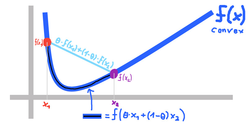
This is usable to define and show convexity of functions analogously to the definition of convex sets.
In probability
If we have a random variable X with probability distribution p(x) over x, then we could set \(x_1=x_2=E[X]\). For this case the Jensen’s inequality displays itself as:
\[f(E[X]) \le E[f(X)]\]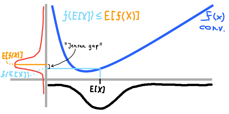
For affine functions f the equality holds. Which tells us that they are concave and convex.
Derivation of the ELBO
\(log p(X)\) is the log evidence, X the observed variables and Z the latent variables. q denotes a variational approximation of p(Z|X):
\[log p(X) = log \int_{Z} p(X,Z)\] \[= log \int_{Z} p(X,Z) \frac{q(Z)}{q(Z)} = log \int_{Z} \frac{p(X,Z)}{q(Z)} q(Z)\]This is the definition of the expected value wrt q(Z):
\[= log(E[\frac{p(X,Z)}{q(Z)}])\]Here comes the inverted Jensen’s inequality in to play (it holds for concave functions). We can confirm ourselves easily that the log() is a concave function by noting that the area under its curve is convex.
\[log(E[\frac{p(X,Z)}{q(Z)}]) \ge E[log( \frac{p(X,Z)}{q(Z)} )]\]This can be brought into a nicer form by realizing that the definition of entropy is \(H(p) = E_{x\sim p(x)}[log(\frac{1}{p(x)})] = -E_{x\sim p(x)}[log ~ p(X)]\)
\[E[log( \frac{p(X,Z)}{q(Z)} )] = E[log(p(X,Z)) - log(q(Z))]\] \[E[log(p(X,Z)) - log(q(Z))] = E[log(p(X,Z))] - E[log(q(Z))]\] \[E[log(p(X,Z))] - E[log(q(Z))] = E[log(p(X,Z))] + H(q(Z))\]Proof Kullback-Leibler divergence is always >= 0
The KL between p(x) and q(x) is defined as:
\[KL(p(x);q(x)) = -E_{x \sim p(x)}[log(\frac{q(x)}{p(x)})]\]We can apply the concave version of Jensen’s inequality. q/p is the distribution and log the concave function.
\[-E_{x \sim p(x)}[log(\frac{q(x)}{p(x)})] \le - log(E_{x \sim p(x)}[\frac{q(x)}{p(x)}])\]Multiply by (-1):
\[E_{x \sim p(x)}[log(\frac{q(x)}{p(x)})] \ge log(E_{x \sim p(x)}[\frac{q(x)}{p(x)}])\] \[log(E_{x \sim p(x)}[\frac{q(x)}{p(x)}]) = log(\int p(x)\frac{q(x)}{p(x)} ~ dx) = log(\int q(x) ~ dx)\]q is a pdf therefore this integral has to be 1. log(1) = 0. As a result:
\[E_{x \sim p(x)}[log(\frac{q(x)}{p(x)})] \ge 0\]