This post explains iDistance and R-Trees for k Nearest Neighbour (kNN) matching. Both are using regular database indices to solve the problem.

Problem

• Assume you want to use kNN in a live system with many data points.
• The data points are rows in your relational database.
• Problem: The classic kNN algorithm would have to scan your whole table.
• Solution: Build an index.

In the following I am going to explain two possible solutions using indices which are implemented in most database systems.

R-Trees

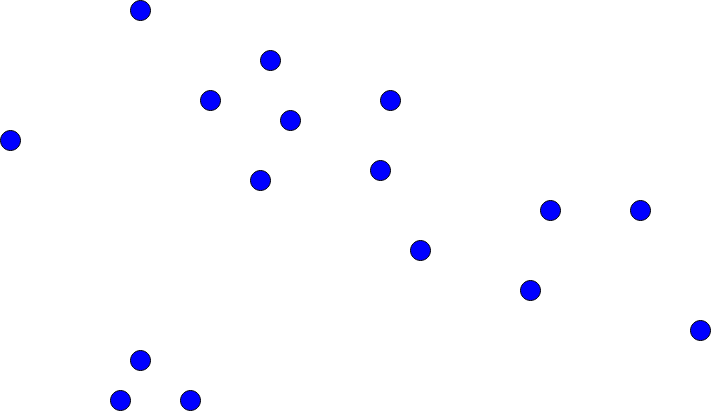
We have the following point cloud:

Now, depending on the exact tree implementation (for example x-tree), the space get separated into multiple layers of containing rectangles. Every rectangle is a minimum bounding rectangle for either another rectangle or points of a lower layer.

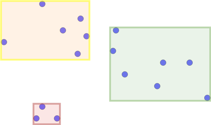
The recursive structure of the rectangles containing rectangles or points forms a tree: the R-tree.

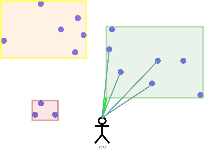
Now let us say that you are here:

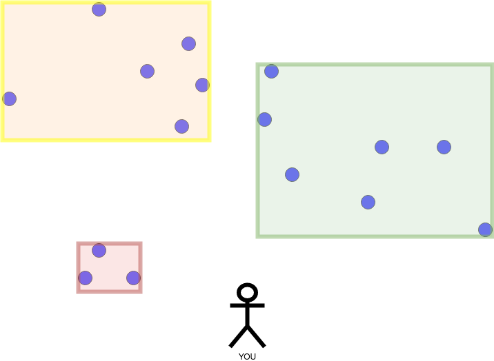
And want to find the k=4 nearest points.

We start by calculating the distance to the closest objects in the highest layer. The highest layer only contains rectangles, therefore we calculate the shortest distance to the rectangles.

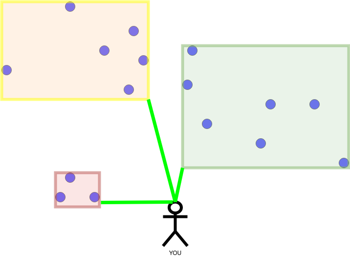
We traverse the rectangles by ascending distance until a rectangle is more distant than our furthest nearest neighbour. All of the points in a rectangle are scanned sequentially.

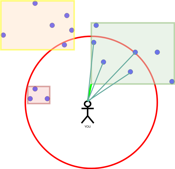
The next image shows the best k=4 candidates.

The largest distance within the group of candidates determines whether we can exclude rectangles. The distance is illustrated as a red circle in the next image.

Having finished the right rectangle. We proceed to the left, small rectangle. The nearest neighbours change, because there are closer ones. This results in a red circle with a smaller diameter.

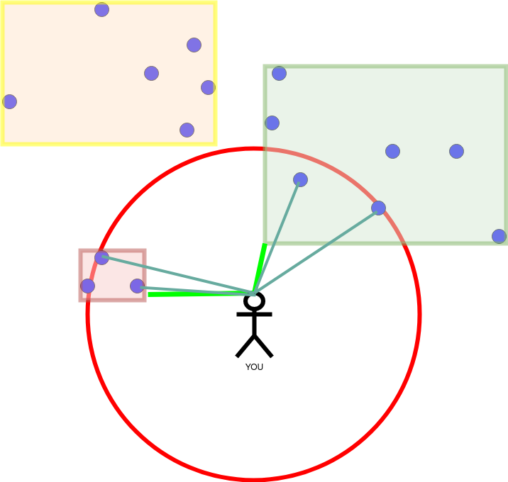
Finished! The yellow rectangle is out of reach. It was not processed but it could neither supply a point close enough to become a nearest neighbour. This “exclusion” is what saves us from doing a whole sequential scan.

The problem with R trees

According to the curse of dimensionality: With increasing dimensionality, the distance between two points grows exponentially.

This results in larger minimum bounding rectangles which tend to span the whole space diagonal. But these rectangles are not a good partitioning of the space anymore. To many intersections between them result in scanning most of them. This can become even worse than the sequential scan, because now we use an index which takes up space, but only supports sequential scans.

iDistance

The main idea of iDistance is to partition the space into spheres. And then reduce the points which have to be scanned by using the distance of the points to their closest sphere center in a B+ tree.

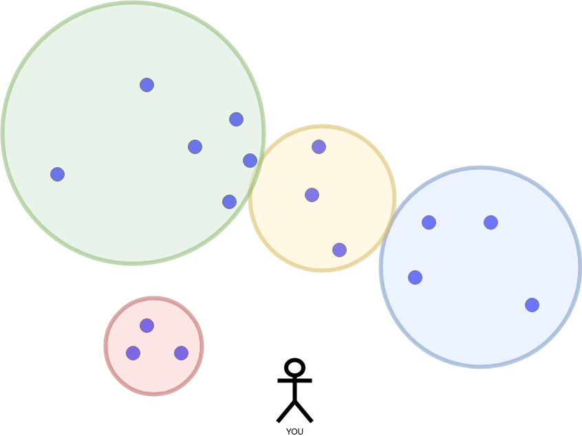
We visualize the algorithm with the following point cloud again. This time we look for k=3.

First of all we have to partition the data. For example using k-Means or DBSCAN.

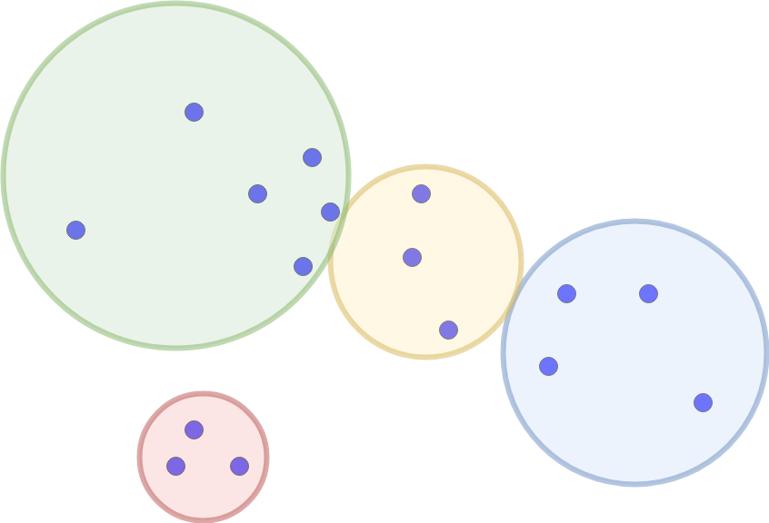
Every point is only part of one partition (sphere). For every partition we calculate the distance to the center and use this information as an index for the partition. This is where the B+ tree is used. (Note: It is also possible to use a single B+ tree for all partitions. It just necessary to shift the centers with an offset large enough to disable intersections. The space diagonal should be enough.)

It is time for a new query at the same position:

Opposed to the procedure of the R trees which shrank the radius of the red circle, iDistance starts with a small radius and increases it incrementally. These are two hyperparameters: initial_radius and radius_growth_factor.

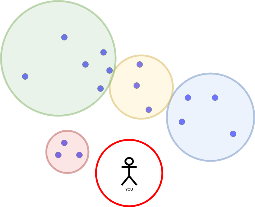
The initial_radius was too small. We found no partition. As long as we don’t have enough points, we increase the initial_radius by multiplying it with the radius_growth_factor.

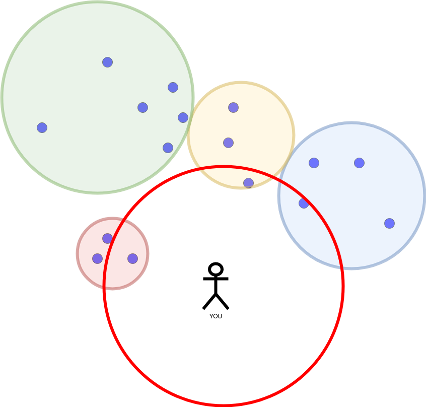
We find three intersections with three partitions. Here comes the “trick”. For every partition we can calculate the ring which intersects with the red query circle. Only the points in the ring can be in the intersection. The rest of the partition does not have to be scanned (marked with black). This saves us time.

In the case of our example for k=3 we would already be done:

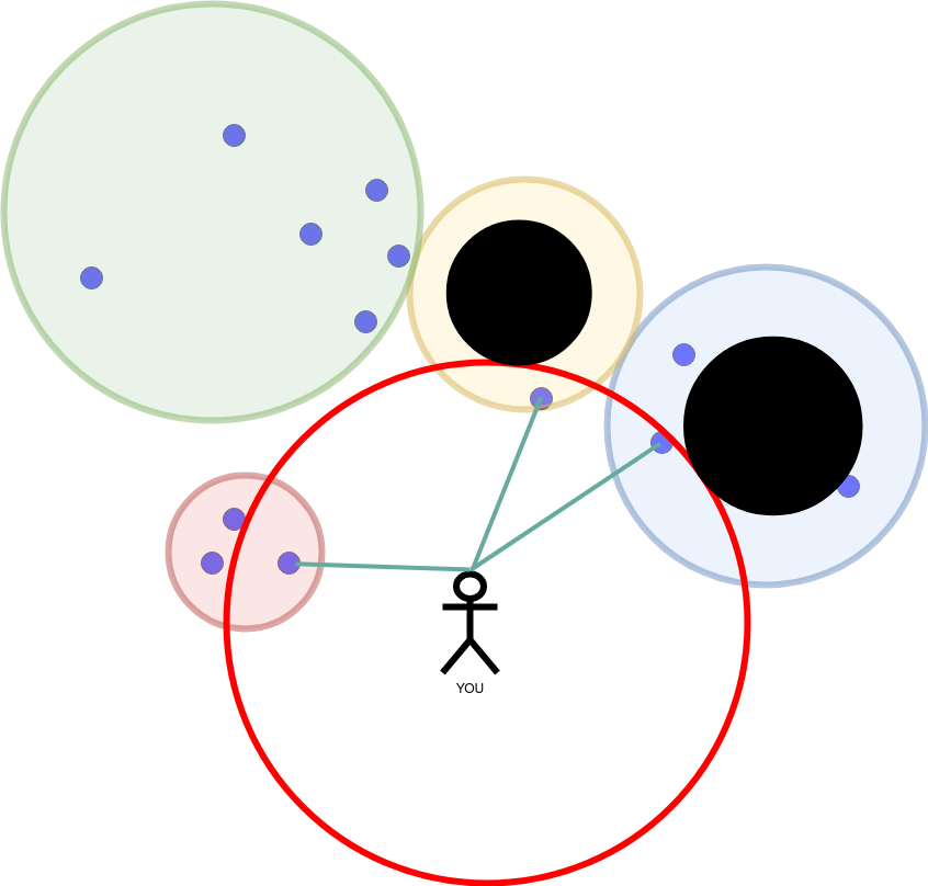
Attention: All points in the ring have to be scanned.

In the case of the left, small circle, another speedup comes in handy, too. The B+ tree of this partition allows us to early abort the search. We can order the points in descending distance from the center. This way we start with the closest point first. Fortunately it is also closest to our point and we can stop the search. Note however, that it does not have to be that way. The point with the largest distance to the center of this partition could also have been on the left side of the center.

iDistance is not a mitigation to the problem introduced by the curse of dimensionality but it can restrict the search space within a partition. This leads to a better behaviour compared to the R tree.