Discrete HMM
We can use a markov chain to model a stochastic process. A popular example is a weather model. We assume that the past can be summed up to states which describe enough to decide which state will be next. Today is rain, tomorrow is also rain. How many steps into the past we take into account describes of which order our Markov Chain is. The simplest Markov Chain is of first order.
But what if we cannot observe the real states? For example we only see whether our room mate leaves the room with an umbrella or sunglasses. It could be that he carries an umbrella with him although there was no rain. Or a classic italian cliche, he uses sunglasses although it is cloudy.
This is a double stochastic process which we can model with a hidden markov model (HMM). As of this writing HMMs are still state of the art in automatic speech recognition. They can be used to estimate the true states of a traffic light (imagine observing a traffic light and from time to time there is a lense flare or a raindrop changing the color of the traffic light for some milliseconds). HMMs can be employed to estimate the driving behaviour of cars or observed agents in general.
A HMM is a five tuple of the following elements:
- States S
- Set of possible Observations V
- Transitions probabilities A
- Emmission probabilities B
- Start probabilities pi
There are three general problems we have to solve for HMMS:
First: Evaluation problem: What is the probability of a sequence of observations O given our HMM: P(O|HMM) Second: Decoding problem: What is the most probable sequence of hidden states q that was traversed to produce the sequence O: P(Q|O,HMM) Third: Training problem: How can we find a better parameters A, B, pi for HMM’ to improve the likelihood of our data: P(O|HMM’) >= P(O|HMM)
Toy data
This blog post explains python/numpy code to solve these problems with the usual algorithms. Our play example will be the mentioned room mate weather model.
import numpy as np


# Example data: inferring weather by room mate's umbrella decisions

# States
rainy = 0
sunny = 1
S = [rainy, sunny]

# Observations
an_umbrella = 0
no_umbrella = 1
V = (an_umbrella, no_umbrella)

# Adjacency: Transition probabilities
A = [
    [0.6, 0.4],
    [0.2, 0.8]
]

# Emissions probabilities
# P(t1=rain \| t0=rain) = 90%
#  -> B[rainy] is the probability distribution
B = [
    [0.9, 0.1],
    [0.2, 0.8]
]

# Start distribution
#  -> 80% for rain
pi = [
    0.8,
    0.2
]
Evaluation problem
There are two algorithms that calculate P(O|HMM) to solve the evaluation problem. They return the same result. The forward algorithm and the backward algorithm. But to gain some intuition on the problem we try to solve the problem in a first step with the naive approach.
Naive approach
Given: HMM lambda, Observervation O (e.g. umbrella, umbrella, no_umbrella) Goal: Compute the likelihood of the observation given the HMM: P(O|HMM).
Let us assume that there is an ideal sequence of hidden states which were traversed to produce the sequence. The probability would be: P(O|Q, HMM) = P(O,Q|HMM) * P(Q|HMM)
This can be rewritten as follows: P(O|Q, HMM) = P(O,Q|HMM) * P(Q|HMM)
The first term P(O,Q|HMM) can be calculated like this: b_q1(o_1) * … * b_qT(o_T) which is the product of correct emmission probabilities. o_1 is the first observation. b_q1(o_1) is the probability that in state q1 the correct symbol was observed. For example: What was the probability that on the first day it was sunny and we observed that our room mate took an umbrella with him. The last thing really happened because we have seen him leave the house with an umbrella.
The second term P(Q|HMM) = pi_q_1 * a_q1,q2 * … * a_q{t-1},qT. Is the probability of the given hidden sequence q. It is just the probability to start in that state and incrementally multiplying with the transition probability to come to the next hidden state in the sequence. For example: We think that q=(rain, rain, rain) then we calculte P(Q|HMM) = 0.8 * 0.9 * 0.9
Key concept: Now we calculate the probability for every single permutation of hidden states. We sum these up which is called a marginalization over q which intuitively means that we “remove” the variable Q from P(O|Q, HMM) => P(O|HMM) which is what we were looking for.
Complexity: Calculate P(O,Q|HMM) for all permutations of N states in T timesteps. N^T calculations. P(O,q|HMM) for a single q we iterate over all timesteps T. => O(T * N^T)
# Given: A hmm and an observation O
# Goal: Compute the likelihood of that observation given the model H
#       P(O\|H)

# We start with the na.ive approach
# Q: the ideal path

# P(O\|Q, HMM) = P(O,Q\|HMM) * P(Q\|HMM)
#                  (a)          (b)

# (a) P(O,Q\|HMM) = b_q1(o_1) * ... * b_qT(o_T)
#
# (b) P(Q\|HMM) = pi_q_1 * a_q1,q2 * ... * a_q{t-1},qT

# Marginalisation: sum over all possible q in Q
# P(O\|Q) = sum over Q: P(O,Q\| HMM)

def all_possible_q(states, sequence_length):
    # Calculate all possible permutations explicitly to see the complexity
    sequence_length -= 1
    if sequence_length == 0:
        return []
    qs = [[s] for s in states]
    for i in range(sequence_length):
        new_seqs = []
        for seq in qs:
            for q in states:
                new_seqs.append(seq + [q])
        qs = new_seqs
    return qs

# Example observations
O = [an_umbrella, an_umbrella, an_umbrella]

# Test the function
all_Q = all_possible_q(S, len(O))

print(all_Q)
[[0, 0, 0], [0, 0, 1], [0, 1, 0], [0, 1, 1], [1, 0, 0], [1, 0, 1], [1, 1, 0], [1, 1, 1]]
def naive_evaluation(A, B, pi, O, S):
    print('Naive forward O='+repr(O))
    all_q = all_possible_q(S, len(O))
    sum_ = 0
    for Q in all_q:
        # p is joint probability P(O,Q\|HMM)
        p = pi[Q[0]] * B[Q[0]][O[0]]
        for t in range(0, len(Q)-1):
            p *= A[Q[t]][Q[t+1]] * B[Q[t+1]][O[t+1]]

        # marginalization
        sum_ += p

    print('P(O\|HMM) = {}'.format(sum_))

    return sum_

# test the evaluation with some examples. A sequence with umbrellas should have the highest probability
p1 = naive_evaluation(A, B, pi, [an_umbrella, an_umbrella, an_umbrella], S)
p2 = naive_evaluation(A, B, pi, [no_umbrella, no_umbrella, no_umbrella], S)
p3 = naive_evaluation(A, B, pi, [no_umbrella, an_umbrella, no_umbrella], S)
p4 = naive_evaluation(A, B, pi, [an_umbrella, no_umbrella, no_umbrella], S)
Naive forward O=[0, 0, 0]
P(O\|HMM) = 0.26728
Naive forward O=[1, 1, 1]
P(O\|HMM) = 0.08752
Naive forward O=[1, 0, 1]
P(O\|HMM) = 0.04848
Naive forward O=[0, 1, 1]
P(O\|HMM) = 0.18568
Forward algorithm
The idea of the forward algorithm is a greedy breadth search. We start in the first time step. Multipply the initial probs pi with the emmission prob b to observe the correct symbol in the state. Now we go to the next time step and calculate the prob alpha for every state. Alpha says: What is the probability to be in this state and having only observed correct symbols. We calculate alpha by summing the alphas of the last states multiplied the the probabilities for a transition to the new state. And then we add the probability to observe the correct symbol in this state.
When we arrive at the last state we sum up all alphas which is P(O|HMM). This make intuitively sense because it is the sum over all sequences that make the correct predictions (compare to the naive approach). The forward algorithm works inductively. (1) init probs, (2) induction step t-1 to t and (3) termination stage at T.
The time complexity can be read from the following code:
- iterate over timesteps T
- calculate alpha for every state s by using the results of all states of T-1 -> S^2
- N = len(States)
=> O(N^2 * T)
# Forward algorithm

def forward_algorithm(A, B, pi, O, S):

    # Init (1)
    alphas = [
        [pi[S[i]] * B[i][O[0]] for i in range(len(S))]
    ]

    # Induction (2)
    for t in range(1, len(O)):
        alphas_t = []
        # Iterate over all state
        for j in range(len(S)):
            sum_ = 0
            # add precessors
            for i in range(len(S)):
                sum_ += alphas[t-1][i] * A[i][j]
            # emissions
            sum_ *= B[j][O[t]]
            alphas_t.append(sum_)

        # save alphas
        alphas.append(alphas_t)

    # termination stage (3)
    p = 0
    for i in range(len(S)):
        p += alphas[-1][i]

    # print('P(O\|HMM) = {}'.format(p))

    return p, alphas


# test the implementation against the naive approach
p5 = forward_algorithm(A, B, pi, [an_umbrella, an_umbrella, an_umbrella], S)
p6 = forward_algorithm(A, B, pi, [no_umbrella, no_umbrella, no_umbrella], S)
p7 = forward_algorithm(A, B, pi, [no_umbrella, an_umbrella, no_umbrella], S)
p8 = forward_algorithm(A, B, pi, [an_umbrella, no_umbrella, no_umbrella], S)

for p_1, p_2 in zip([p1, p2, p3, p4], [p5, p6, p7, p8]):
    print('Same? {} {} '.format(p_1, p_2[0]))
Same? 0.26728 0.26728
Same? 0.08752 0.08752
Same? 0.04848 0.04848
Same? 0.18568 0.18568
Backward algorithm
The second option to evaluate is recursive. For every hidden state unrolled over time we compute a beta. The beta stores the probability that only correct observations are going to be made after this state.
In the last timestep T we can say that all betas are 100% because no observation is going to come afterwards so there won’t be a mistake. (1)
The next step (2) is to recurse from t+1 to t. We can calculate the beta for t by summing over all states at t+1 multiplied by their transition prob and the emission prob.
Termination (3): The betas at the first time steps differ slightly because we use the pis instead of transitions probs. Then we sum over all the first betas which gives us P(O|HMM).
Forward and backward algorithm have the same complexity.
def backward_algorithm(A, B, pi, O, S):

    # Init (1)
    betas = [
        [1 for i in range(len(O))]
    ]

    # Recursion (2)
    # go from t=T to t=1
    for t in range(0, len(O)-1)[::-1]:
        betas_t = []

        # for all states in t
        for i in range(len(S)):
            sum_ = 0

            # sum over all successors
            for j in range(len(S)):
                sum_ += A[i][j] * B[j][O[t+1]] * betas[-1][j]

            betas_t.append(sum_)

        betas.append(betas_t)

    # Termination (3)
    p = 0
    for j in range(len(S)):
        p += pi[j] * B[j][O[0]] * betas[-1][j]

    return p, betas[::-1]

# test the implementation against the naive approach
p9 = backward_algorithm(A, B, pi, [an_umbrella, an_umbrella, an_umbrella], S)
p10 = backward_algorithm(A, B, pi, [no_umbrella, no_umbrella, no_umbrella], S)
p11 = backward_algorithm(A, B, pi, [no_umbrella, an_umbrella, no_umbrella], S)
p12 = backward_algorithm(A, B, pi, [an_umbrella, no_umbrella, no_umbrella], S)

for p_1, p_2, p_3 in zip([p1, p2, p3, p4], [p5, p6, p7, p8], [p9, p10, p11, p12]):
    print('Same? {} {} {}'.format(p_1, p_2[0], p_3[0]))
Same? 0.26728 0.26728 0.26728
Same? 0.08752 0.08752 0.08752
Same? 0.04848 0.04848 0.04848
Same? 0.18568 0.18568 0.18568
Decoding
Maybe you wondered why we implemented both, the forward and backward algorithm although they have equivalent results. The answer: We want to use the alphas and betas for naive decoding and the training problem.
So what was the decoding problem? Given a sequence of observations O, what sequence of hidden states produced our observation with the highest probability?
There are two possible optimality criteria:
- Sequence of maximum likely single states “Forward-Backward-Algorithm”
- Maximum likely sequence “viterbi algorithm”
Forward-Backward-Algorithm
First let us take a look at the forward backward algorithm. For every timestep we want to pick the state which is most likely. Therefore we define gammas for every state unrolled over time. The gamma calculates the prob for every single state P(q_t = S_i| O, HMM).
Using the product rule we transform the term: P(q_t=S_i, O|HMM) / P(O|HMM) P(O|HMM) was the result of the evaluation problem. We divide by it so our gammas are normalized to a probability distribution.
Key concept: The prob that state S_i is part of the optimal state sequence P(q_t=S_i, O|HMM) = alpha_t(S_i) * beta_t(S_i). And that is really interesting. alpha*beta for the state S_i means: probability of having observed only correct things and going to observe only correct things. For a given time steps all states have different gammas and we just pick the highest. => q_t = arg_i max gamma(i)
Complexity of the following code: forward O(N^2 * T) + backward O(N^2 * T) + gammas O(TN) + argmax O(NT) ~= O(2N^2T+2NT) part of N^2.
def forward_backward_algorithm(A, B, pi, O, S):
    p, alphas = forward_algorithm(A, B, pi, O, S)
    p, betas = backward_algorithm(A, B, pi, O, S)

    gammas = []

    # for every timestep
    for t in range(len(O)):
        gammas_t = []

        sum_ = 0

        # for every state
        for i in range(len(S)):
            gammas_t.append(alphas[t][i] * betas[t][i])
            sum_ += gammas_t[-1]

        # normalize gammas to make them a prob distribution
        for i in range(len(S)):
            gammas_t[i] /= sum_

        gammas.append(gammas_t)

    seq = []

    # find max of gamma for every timestep
    for t in range(len(O)):

        # stupid argmax
        max_ = 0
        max_index = -1
        for i in range(len(S)):
            if gammas[t][i] > max_:
                max_ = gammas[t][i]
                max_index = i

        seq.append(max_index)

    return seq, gammas

# test: the adjacency matrix has high probabilities for rain to stay.
# That means that a single day of rain is not really probable.
# -> the following sequence should be all sunny
#    except for the last state because it is more probable that after umbrella comes another umbrella
#    which would be rainy.

O = [no_umbrella, no_umbrella, an_umbrella] * 10

path, gammas = forward_backward_algorithm(A, B, pi, O, S)

print(path)
[1, 1, 1, 1, 1, 1, 1, 1, 1, 1, 1, 1, 1, 1, 1, 1, 1, 1, 1, 1, 1, 1, 1, 1, 1, 1, 1, 1, 1, 0]
Viterbi-Algorithm
The problem of the forward backward algorithm is that it treats the states as individuals but they are not. They should be viewed in their context. For example with their next neighbours. But in most scenarios it would be the best idea to use the whole sequence. This way the problems of the Forward-Backward-Algorithm can be mitigated. A problem is that two succinct states can have the highest gammas but have a transition probability of zero between them. Such sequences cannot be the most probable ones.
Taking the full sequence into account is what the viterbi algorithm does. An illustrative example for the viterbi. Imagine you are planning a roadtrip from the West Coast of the United States to the East Coast. You divide the country into vertical stripes with the same width and choose some cities for every stripe in the state. For every day of your road trip you want to advance by one stripe but if you can choose you prefer to drive as little as possible. Which means: The probability of you taking the shorter highway is higher than the longer one. To solve this problem with viterbi we have to know that viterbi works nearly the same as the forward algorithm but instead of taking the sum over the precessors we take the maximum and store a backpointer.
Superb viterbi roadtrip: https://www.youtube.com/watch?v=6JVqutwtzmo
So: Every city at the West coast is equally probable. Then we go to the next stripe. For every city in this stripe we calculate the pairwise distance to the cities of the west coast, store the smallest distance and store a backpointer to remember which street we would take from this city to go backwards. We repeat this until we can reach every city of the East coast. Now we just pick the one with the lowest accumulated miles on its path, collect its backpointers and return the reversed list of backpointers.
Back to the implementation: As with the forward algorithm we define deltas to store the bast accumulated probabilities in a given state in time (the miles to reach a city of any stripe). We init (1) them with the initial probs pi times the correct observation. Then we have an induction step (2) which sets the backpointer (psi) for every state t+1 to state t.
In the termination step (3) we max the arg max on the deltas of timestep T and collect the backpointers.
def viterbi(A, B, pi, O, S):
    # init (1)
    deltas = [
        [pi[S[i]] * B[S[i]][O[0]] for i in range(len(S))]
    ]

    # backpointer through trellis
    psis = [
        [0 for i in range(len(S))]
    ]

    # induction (2)
    # for every timestep
    for t in range(1, len(O)):
        deltas_t = []
        psis_t = []

        # for every state
        for j in range(len(S)):
            max_delta = float('-inf')
            backptr = -1

            # for every state
            for i in range(len(S)):
                delta = deltas[t-1][i] * A[S[i]][S[j]]
                if delta > max_delta:
                    max_delta = delta
                    backptr = i

            deltas_t.append(max_delta * B[S[j]][O[t]])
            psis_t.append(backptr)

        deltas.append(deltas_t)
        psis.append(psis_t)

    # arg max delta at last timestep
    max_t = float('-inf')
    max_i = -1
    for i in range(len(S)):
        if deltas[-1][i] > max_t:
            max_i = i
            max_t = deltas[t][i]

    q_t = max_i

    # Termination (3)
    path = []
    for t in range(len(O))[-1::-1]:
        q_t = psis[t][q_t]
        path.append(q_t)

    return path[::-1]

# test
path = viterbi(A, B, pi, O, S)
print(path)
[0, 1, 1, 1, 1, 1, 1, 1, 1, 1, 1, 1, 1, 1, 1, 1, 1, 1, 1, 1, 1, 1, 1, 1, 1, 1, 1, 1, 1, 1]
# compare naive and viterbi

Os = [
    [no_umbrella]*5,
    [an_umbrella]*5,
    [an_umbrella, no_umbrella]*5,
    [no_umbrella, an_umbrella]*5,
    [no_umbrella, no_umbrella, an_umbrella]*5,
    [no_umbrella]*5 + [an_umbrella]*5 + [no_umbrella]*5,
]

for O in Os:
    print('-'*80)

    path1, _ = forward_backward_algorithm(A, B, pi, O, S)
    path2 = viterbi(A, B, pi, O, S)

    print('Observations:')
    print(O)
    print('\n')
    print('Naive \t \| Viterbi \t \| same?')
    print('-'*40)
    for q_a, q_b in zip(path1, path2):
        print('{} \t \| {} \t\t \| {}'.format(q_a, q_b, q_a == q_b))

    print('\n'*5)
--------------------------------------------------------------------------------
Observations:
[1, 1, 1, 1, 1]


Naive 	 \| Viterbi 	 \| same?
----------------------------------------
1 	 \| 0 		 \| False
1 	 \| 1 		 \| True
1 	 \| 1 		 \| True
1 	 \| 1 		 \| True
1 	 \| 1 		 \| True


--------------------------------------------------------------------------------
Observations:
[0, 0, 0, 0, 0]


Naive 	 \| Viterbi 	 \| same?
----------------------------------------
0 	 \| 0 		 \| True
0 	 \| 0 		 \| True
0 	 \| 0 		 \| True
0 	 \| 0 		 \| True
0 	 \| 0 		 \| True


--------------------------------------------------------------------------------
Observations:
[0, 1, 0, 1, 0, 1, 0, 1, 0, 1]


Naive 	 \| Viterbi 	 \| same?
----------------------------------------
0 	 \| 0 		 \| True
1 	 \| 0 		 \| False
1 	 \| 1 		 \| True
1 	 \| 1 		 \| True
1 	 \| 1 		 \| True
1 	 \| 1 		 \| True
1 	 \| 1 		 \| True
1 	 \| 1 		 \| True
1 	 \| 1 		 \| True
1 	 \| 1 		 \| True


--------------------------------------------------------------------------------
Observations:
[1, 0, 1, 0, 1, 0, 1, 0, 1, 0]


Naive 	 \| Viterbi 	 \| same?
----------------------------------------
1 	 \| 0 		 \| False
0 	 \| 1 		 \| False
1 	 \| 1 		 \| True
1 	 \| 1 		 \| True
1 	 \| 1 		 \| True
1 	 \| 1 		 \| True
1 	 \| 1 		 \| True
1 	 \| 1 		 \| True
1 	 \| 1 		 \| True
0 	 \| 1 		 \| False


--------------------------------------------------------------------------------
Observations:
[1, 1, 0, 1, 1, 0, 1, 1, 0, 1, 1, 0, 1, 1, 0]


Naive 	 \| Viterbi 	 \| same?
----------------------------------------
1 	 \| 0 		 \| False
1 	 \| 1 		 \| True
1 	 \| 1 		 \| True
1 	 \| 1 		 \| True
1 	 \| 1 		 \| True
1 	 \| 1 		 \| True
1 	 \| 1 		 \| True
1 	 \| 1 		 \| True
1 	 \| 1 		 \| True
1 	 \| 1 		 \| True
1 	 \| 1 		 \| True
1 	 \| 1 		 \| True
1 	 \| 1 		 \| True
1 	 \| 1 		 \| True
0 	 \| 1 		 \| False


--------------------------------------------------------------------------------
Observations:
[1, 1, 1, 1, 1, 0, 0, 0, 0, 0, 1, 1, 1, 1, 1]


Naive 	 \| Viterbi 	 \| same?
----------------------------------------
1 	 \| 0 		 \| False
1 	 \| 1 		 \| True
1 	 \| 1 		 \| True
1 	 \| 1 		 \| True
1 	 \| 1 		 \| True
0 	 \| 1 		 \| False
0 	 \| 0 		 \| True
0 	 \| 0 		 \| True
0 	 \| 0 		 \| True
0 	 \| 0 		 \| True
1 	 \| 0 		 \| False
1 	 \| 1 		 \| True
1 	 \| 1 		 \| True
1 	 \| 1 		 \| True
1 	 \| 1 		 \| True
Training problem
The problems are sorted by their difficulty. For the evaluation problem we can give a probability. For the decoding problem it is not that clear how to calculate the optimal sequence q. What about training? Here we also have to define optimality.
If we are looking for parameters that maximize the likelihood of the observations we can use EM training. The Baum-Welch-Algorithm (BW) is a solution to iteratively reestimate the parameters of the HMM. BW turned out to be a special form of expectation maximization (EM). BW is generative learning. Which means that the HMM learns the “shape” of the sequences and is able to produce new sequences with high likelihoods. But if we want to use the HMM for disriminating only (in automatic speech recognition we care about classifying MFCC vectors to 100 - 200 phonemes). Then we can use the Extended-Baum-Welch-Algorithm (EBW) which allows us to do discriminate learning. The result is that the HMM not only uses the positive samples but also the negative samples and to maximize the distance between the two classes. In ASR we observe something like a spoken sentence. We have as transcription of the sentence. But we want to know what phonemes produced the audio signal. These are our hidden states. Speech recognition systems are evaluated by the word error rate but the BW maximizes the full sequence therefore it tries to minimize the sentence error rate. We can bring this together with the EBW which minimizes the WER.
Let’s get back to the simple practical examples. How does BW work?
Repeat:
- Compute an auxilary function Q (Baum’s auxilary function) which is a proxy for the log likelihood of the model. If Q increases, so does P(O|HMM). Q(HMM, HMM’) = \sum_{Q}{ P(Q|O, HMM) * log( P(O,Q|HMM’) }
- arg max Q => better or equally good HMM’
How can we just “arg max” Q? This can be done by gradient descent which is slow and has the known problems. Or it can be done as a constrained optimization problem (Lagrange multiplier). The constraints are that the new parameters have to be probability distributions again (sum up to one).
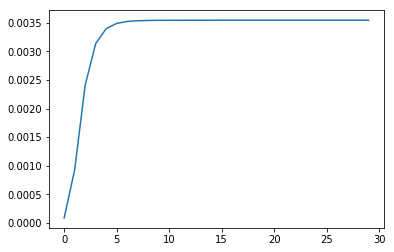
The bottom line: Baum and his team came up with formulas for reestimation of parameters with P(O|HMM’) >= P(O|HMM) ! So just initialize randomly and iterate until we don’t get better.
# Baum-Welch-Regeln

def train(A, B, pi, O, S, V):
    p_observation, alphas = forward_algorithm(A, B, pi, O, S)
    p_observation2, betas = backward_algorithm(A, B, pi, O, S)

    # these are the same gammas as in the forward-backward algorithm
    gammas = []
    for t in range(len(O)):
        gammas_t = []
        sum_ = 0
        for i in range(len(S)):
            gammas_t.append(alphas[t][i] * betas[t][i])
            sum_ += gammas_t[-1]
        for i in range(len(S)):
            gammas_t[i] /= sum_
        gammas.append(gammas_t)

    # xsi is the probability of taking a transition from one state to another
    # and observing the correct symbols
    xsis = []
    for t in range(len(O)-1):
        xsis_i = []
        for i in range(len(S)):
            xsis_j = []
            for j in range(len(S)):
                sum_ = 0
                for i2 in range(len(S)):
                    for j2 in range(len(S)):
                        sum_ += alphas[t][i2] * A[i2][j2] * B[j2][O[t+1]] * betas[t+1][j2]
                numerator = alphas[t][i] * A[i][j] * B[j][O[t+1]] * betas[t+1][j]
                xsis_j.append(numerator/sum_)
            xsis_i.append(xsis_j)
        xsis.append(xsis_i)

    # the reestimated pis are just the gammas.
    # Gamma is the probability of being in a state
    pi_improved = [gammas[0][i]  for i in range(len(pi))]

    #         expected number of transitions from State i to j
    # a_ij =  ------------------------------------------------
    #           expected number of transitions from State i

    A_improved = []
    for i in range(len(S)):
        A_i = []
        for j in range(len(S)):
            gamma_sum = 0
            xsi_sum = 0
            for t2 in range(len(O)-1):
                gamma_sum += gammas[t2][i]
                xsi_sum += xsis[t2][i][j]
            A_i.append(xsi_sum/gamma_sum)
        A_improved.append(A_i)

    #             expected number of times in state j and observing k
    # b_j (k) = --------------------------------------------------------
    #                expected number of times in state j

    B_improved = []

    for j in range(len(B)):
        b_j = []
        for k in range(len(V)):
            expected_number_in_state_j_with_vk = 0
            exp_num_times_in_state_j = 0
            for t in range(len(O)):
                if O[t] == V[k]:
                    expected_number_in_state_j_with_vk += gammas[t][j]
                exp_num_times_in_state_j += gammas[t][j]

            b_j_k = expected_number_in_state_j_with_vk / exp_num_times_in_state_j

            b_j.append(b_j_k)

        B_improved.append(b_j)

    return A_improved, B_improved, pi_improved, p_observation
p_statistics = []

A_, B_, pi_, p = train(A, B, pi, O, S, V)
for _ in range(30):
    p_statistics.append(p)
    A_, B_, pi_, p = train(A_, B_, pi_, O, S, V)
    # print('P(O\|HMM)={}'.format(p))
import matplotlib.pyplot as plt

plt.plot(p_statistics)
plt.show()
O
[1, 1, 1, 1, 1, 0, 0, 0, 0, 0, 1, 1, 1, 1, 1]
pi_
[3.0869536244290596e-210, 1.0]
A_
[[0.8000000000000703, 0.19999999999992943],
 [0.11111111111120028, 0.8888888888887997]]
B_
[[0.999999999999344, 6.559403577247279e-13], [1.264606883900921e-20, 1.0]]
Random Walk
To end this post. Let’s generate “new” sequences from the HMM.
import random
random.seed(42)

for n in range(10):
    random_start = random.random()
    state_sequence = []
    state_sequence.append(int(random_start > pi_[0]))

    for i in range(10):
        state_sequence.append(int(random.random() > A_[state_sequence[-1]][0]))

    observation_sequence = []
    for state in state_sequence:
        observation_sequence.append(int(random.random() > B_[state][0]))

    print(observation_sequence)
[1, 0, 0, 0, 0, 0, 1, 0, 0, 0, 0]
[1, 1, 1, 1, 0, 0, 1, 1, 1, 1, 1]
[1, 1, 0, 0, 0, 0, 0, 0, 0, 1, 1]
[1, 0, 0, 0, 0, 1, 1, 1, 1, 1, 1]
[1, 0, 0, 0, 0, 0, 0, 0, 1, 1, 1]
[1, 1, 1, 1, 1, 1, 1, 1, 1, 1, 1]
[1, 1, 0, 0, 0, 0, 0, 0, 0, 0, 0]
[1, 1, 1, 1, 1, 1, 0, 0, 0, 1, 1]
[1, 1, 1, 1, 1, 1, 1, 0, 0, 0, 1]
[1, 1, 1, 1, 1, 1, 1, 1, 1, 0, 0]