Calculating a feed forward network by hand

In computer science the building blocks of everything are ones and zeros. This simplicity is not an obstacle for building complex systems.

For Artifical Neural Networks the simple building blocks are the perceptrons.

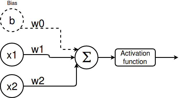
They work by weighting their inputs (w_0, w_1, ..., w_n), summing them up (Σ) and applying an activation function to the output.

Multiple perceptrons form layers and the layers form a neural network. Neural networks are general function approximation machines. That means that for every continuous function within a limited range a neural network can serve an approximation with an error less than some epsilon.

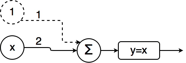
Let’s look at an example with only one perceptron to understand why we want to use them in layers.

Imagine you wanted to approximate f(x) = 2x + 1:

It is easy to see that the following perceptron acts like a linear equation and can be extended to represent the general form of a linear equation system \(Ax + b = y\) by adding more inputs and weights.

But what about non-linear functions

Like f(x) = x^2?

One could propose a network like this:

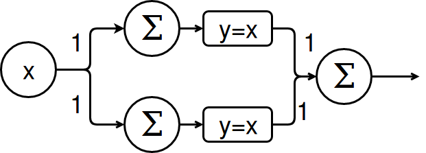
Or even more complex ones but chaining multiple perceptrons together will just mimic another linear equation system as long as the activation function is only linear (y = x).

The first choice for the activation function would be the cubic function itself. But I think approximating a function by using itself is not a valid solution.

Activation functions

There are a lot activation functions like sigmoid, tanh or linear. The default recommendation as of the deeplearningbook is ReLU (rectified linear unit). You can play around with neural networks and different activation functions at: playground.tensorflow.org.

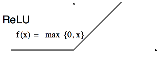
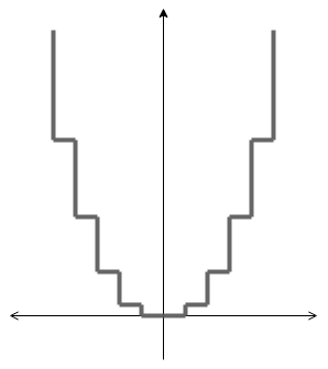
Back to the question: How can a combination of linear functions (ReLU is still linear from -inf to ]0 and ]0 to +inf) approximate a cubic functions?

Well it is definetely not the most precise way to do it but the network could learn a step function like such because the ReLU can “activate” and “deactivate” whether the output of a perceptron shall be used.

Learning XOR

Learning the XOR function was a prominent example of what could not be approximated by a linear model. The following link (playground with linear activation) brings you to the playground of tensorflow. It contains the XOR classification problem and I preset the linear activation function.

It doesn’t matter how many epochs you are going to wait or how many hidden layers you add, the loss will always stay at around 0.5.

But if you switch the activation function to ReLU or anything else and add one hidden layer with four perceptrons you obtain a really good solution.

Calculation

These networks are called feed forward because there is no backward loop as in recurrent neural networks. The perceptrons a. k. a. neurons are illustrated as single units but we are going to deal with them layerwise as vectors.

The following net shall be our example to solve XOR (layout taken from this youtube video):

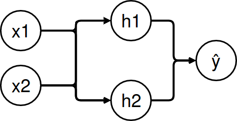
The calculation of every layer i consists of:

• Our input \(x_i\) is a vector. For example: \(x_0 = (0,0)^T\) for the first layer
• The weight matrix \(W_i\)
• The vector of biases for every neuron \(b_i\)
• Estimated values ŷ which are calculated by \(ŷ_i = \sigma ( W_i x_i + b_i )\)
• \(\sigma\) is the activation function

After the first layer the estimated values ŷ are used as inputs for the next layer and so on.

This post won’t explain how to train a neural network. It will only show how to feed the input values through the network to return a prediction (feed forward).

Therefore we assume the following values: **First and seconds weight matrix **

\(W_{1} \begin{pmatrix}20 & 20\\\ -20 & -20\end{pmatrix}\) \(W_{2} \begin{pmatrix}20 & 20 \end{pmatrix}\)

First and second bias vector

\(b_{1} \begin{pmatrix} -10\\\ 30\end{pmatrix}\) \(b_{2} \begin{pmatrix} -30 \end{pmatrix}\)

Let’s calculate the outputs for every possible input:

\[\sigma (\begin{pmatrix}20 & 20 \end{pmatrix} * \sigma \bigg( \begin{pmatrix}20 & 20\\\ -20 & -20\end{pmatrix} * \begin{pmatrix}0\\\ 0\end{pmatrix} + \begin{pmatrix}-10\\\ 30\end{pmatrix} \bigg) + \begin{pmatrix}-30 \end{pmatrix}) = 0\] \[\sigma (\begin{pmatrix}20 & 20 \end{pmatrix} * \sigma \bigg( \begin{pmatrix}20 & 20\\\ -20 & -20\end{pmatrix} * \begin{pmatrix}0\\\ 1\end{pmatrix} + \begin{pmatrix}-10\\\ 30\end{pmatrix} \bigg) + \begin{pmatrix}-30 \end{pmatrix}) = 1\] \[\sigma (\begin{pmatrix}20 & 20 \end{pmatrix} * \sigma \bigg( \begin{pmatrix}20 & 20\\\ -20 & -20\end{pmatrix} * \begin{pmatrix}1\\\ 0\end{pmatrix} + \begin{pmatrix}-10\\\ 30\end{pmatrix} \bigg) + \begin{pmatrix}-30 \end{pmatrix}) = 1\] \[\sigma (\begin{pmatrix}20 & 20 \end{pmatrix} * \sigma \bigg( \begin{pmatrix}20 & 20\\\ -20 & -20\end{pmatrix} * \begin{pmatrix}1\\\ 1\end{pmatrix} + \begin{pmatrix}-10\\\ 30\end{pmatrix} \bigg) + \begin{pmatrix}-30 \end{pmatrix}) = 0\]

The results are exactly how we expect them to be. The original problem of a non-linear function can also be solved in other ways for example with the kernel trick which moves the non-linear function in another dimensionality where it becomes linear. Our network can be interpreted in the same way. The first layer projects the XOR function into another space. The perceptron in the output layer can then learn the parameters of its linear model to discriminate the two classes.