Optimization

Search for the optimum

Assume we define a function f which takes a profession and returns the annual salary. It sounds naturally to search for the optimum. Maybe we even have some constraints like “the job should be in Europe” or “I want to work 30 hours per week”. This is a so called optimization problem.

We define:

• Variables to optimize
• A criteria function which depends on the variables
• Constraints that have to be satisfied by the solution

There exists the general dichotomization into static and dynamic optimization. In static opt. the variables are parameters whereas in dynamic optimization the variables are functions themselves. The criteria function then is a function of a function which has the name functional. A general example for a functional is the integral from zero to one of a function f. It maps the function to a scalar. Control in robotics is mostly dynamic. Classifiying images or speech signals belongs to the static class.

There is the general possibility to find extrema by differentiating and finding the zeros of it. This is done in the Lagrangian method or in a probability context with the Maximum Likelihood estimation.

The term search refers to the attempt of finding a feasible point that satisfies all constraints and yields the lowest possible error (in the example of the beginning this would be the highest salary). Mathematically speaking this is expressed with \(\operatorname*{argmin}_\theta f(x)\) plus some constraints.

Local search starts from a point (a solution) and searches its neighbours for a better solutions which can be optimized again.

Global search: The state space gets evaluated (not only locally) in order to find an optimum. Example: Dynamic Programming

Stochastic search: Finding a new solution involves a nondeterministic component. Like a randomized search in ML.

Uninformed search: All of the options and permutations of them have to be covered. We can’t discard a path until we have tried it out. Breadth-first or depth-first search are examples of this scheme in graphs.

Informed search: Contrary to the uninformed search we use some kind of heuristic to guide the process of obtaining a new solution. The heuristic might exclude parts of the state space so we don’t have to search there. An example is the A* algorithm or the dijkstra. This is related to the global search.

Convex optimization

Linear least squares is the method of finding a line that best fits given data points. “Best fit” means that the sum of the squared distances between a point and the line is minimal. The vertical distance between the point and the line gets called residual.

We assume the observations y are generated by a linear relationship (m) with the data X which is affected by white noise e.

import numpy as np
import matplotlib.pyplot as plt

n = 100
X = np.random.uniform(0, 5, n)
y = 0.3 * X + 2 + np.random.normal(0, 0.1, n)

plt.scatter(X, y)

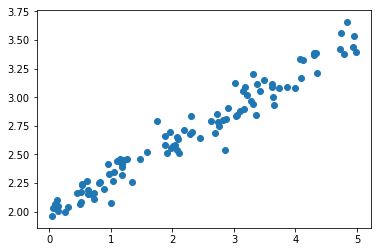
The process that generates the data has two unknown variables \(m\) and \(t\). If the error was not present we could solve for the perfect solution in with two points:

In reality we cannot rely on the data nor can we rely on our model. Therefore we want to use as many points as possible. We just assume that the error has no bias, because we want to take the average of all estimates.

This idea is captured in the Linear least squares:

This is called the quadratic error term. We “search” parameters m and t that minimize the error.

Let’s see how the error term behaves for different values:

ts = np.linspace(-100, 100, 100)
ms = np.linspace(-100, 100, 100)

cost_fn = lambda m, t: np.sum( np.square( y - m*X + t ) )

cost = []
for t in ts:
    cost.append( [cost_fn(m, t) for m in ms] )
    
cost = np.log(np.array(cost))

tt, mm = np.meshgrid(ts, ms)

plt.contourf(tt, mm, cost)
plt.xlabel("t")
plt.ylabel("m");

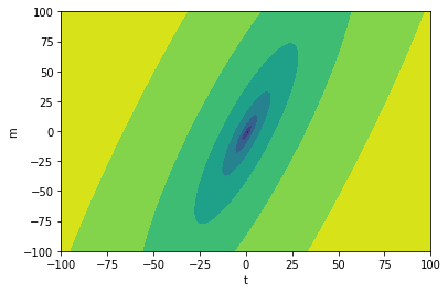
From the equation of the error and the plot, we see that this is a paraboloid. Its curve belongs to the class of convex curves. Finding the optimum is straightforward:

Before doing this we switch to the matrix vector notation because we can handle the sum better in that way.

\(X = (x_1, ..., x_n)^T\) where \(x_i\) is a 2d vector because we add a “1” with the bias trick. For example \(x_i = (1, 2.3)^T\)

\(w = (t, m)^T\) (“weight vector”)

We want to solve for the parameters w:

For the “normal” case where X is a non-square matrix we can use the Moore-Penrose Pseudoinverse with alpha=0:

Note: The result can be proven by differentiating, setting it to zero. \(X\) has to be of full column rank, or else the \(X^T X\) would not be invertible.

Let’s apply this closed form solution to the data:

X_bias = np.vstack([np.ones(X.shape[0]), X]).T
X_bias[:5]

array([[1.        , 4.79006299],
       [1.        , 3.30198279],
       [1.        , 0.63063158],
       [1.        , 1.58619112],
       [1.        , 3.48292161]])

np.matmul(
    np.linalg.inv(
        np.matmul(
            X_bias.T, 
            X_bias)
    ), X_bias.T
).dot(y)

array([1.99713 , 0.302953])

This is really close to the original parameters 2.0 and 0.3.

The “goodness” of the ordinary least squares is proven in the Gauss-Markov Theorem under the assumptions that X has full column rank, the noise is white, the noise per dimensions all have the same variance and they are uncorrelated. The assumptions about the noise signify that the Covariance Matrix of the noise is a diagonal matrix which is scaled by one single factor.

It is the best linear unbiased estimator (BLUE) and this estimator is unique.

Under the assumtion that the noise is normally distributed with a expectation value of zero the method of linear least squares is the same as the linear regression.

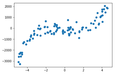
Polynomial regression

The concept of the linear regression can be extended to non-linear curve fitting with a simple trick. We transform the data points \(X\) into its higher polynomials, perform the usual least sqaures fitting and use the parameters in the higher order model.

X = np.random.uniform(-5, 5, n)
y = X**5 + np.random.normal(0, 300, n)

plt.scatter(X, y);

# We treat the polynomials as new dimensions in our data matrix X
X_poly = np.vstack([X**0, X, X**2, X**3, X**4, X**5, X**6, X**7, X**8]).T

# The linear regression from above
beta = np.matmul(
    np.linalg.inv(
        np.matmul(
            X_poly.T, 
            X_poly)
    ), X_poly.T
).dot(y)

beta

array([-1.42284625e+02, -5.03193657e+01,  1.79237377e+01,  3.62618409e+00,
       -2.23686147e+00,  1.87793816e+00,  2.53151667e-01, -4.53556005e-02,
       -8.67038500e-03])

y_2 = [sum([beta[i]*x**i for i in range(len(beta))]) for x in X]

plt.scatter(X, y_2)
plt.scatter(X, y);

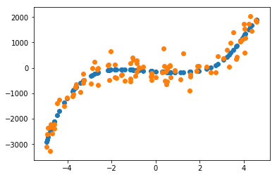
We note that the original parameters were not restored. This is due to the fact that the polynomials are highly correlated and different polynomials can form similar curves.

There is a lot more to say about regression but this text is about optimization which is the reason why I continue with the next topic.

Optimization under constraints

Let’s go through an example: You want to throw a ball over a wall with as little effort as possible. The ball flies in a parabola. You stand at (x=-5, y=0). The wall is at x=0 with a height of 2.

plt.scatter(X, -0.08*X*X + 2.05)
plt.scatter(np.zeros(20), np.linspace(0, 2, 20))

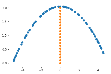
The function we want to maximize is the inverse of the parabola because we want it to be as low as possible:

… (ToDo: Find better example)

These problems were all static optimization problems:

1. Linear opt: linear cost function, linear constraint
2. Quadratic optim.: quadratic cost function, linear constraint
3. Nonlinear optimization: either cost function or a constraint are non linear

Nonlinear optimization

As long as the criteria function f(x) is linear it can be written in linear algebra as a matrix vector product: \(Ax\). Solving these problems comes down to inverting a matrix. There are different ways to do this. It depends on the size of the matrix and its conditioning. For most of the modules availabe these days LAPACK/BLAS takes care of this.

What can we do if we are facing a nonlinear function? Such a term appears for example in the loss function of neural networks.

Performing local search (which is always iterative): In this case we sample the value of the error function at the initial point. We could sample a neighbouring point assuming continuity of the function and calculate the difference quotient. But this does not work in practice because of numerical imprecisions.

What we do instead is to calculate the gradient with backpropagation in our sampled point.

Why should the gradient be of any interest? A short answer might be: We assumed continuity and therefore we can execute a step into the opposite direction (compare this to the Forward-Euler).

A longer answer: What we do by using the gradient is that we linearize the nonlinear error surface around our sampled point (we assume the neighbourhood to be a plane). This is a standard linearization which can be justified by the Taylor approximation. The higher order terms are omitted. So the gradient tells us if we make an infinitesimal step into its direction whether the error will be higher or lower.

Of course the local linearity is not always given. In theory we could for example determine whether a function is Lipschitz-continuous but what would this change? Maybe descrease the step size of gradient descent…

Another option is Newton’s method which involves the second order of the taylor series expansion. With this method we can make faster progress in flat areas (because we now assume that the error is quadratic) but in general it does not help with arbitrary functions. The Hessian can be used to get the curvature of the surface around the point (conditioning number).

Calculating the Hessian is resource intense. The Gauss Newton method approximates the Hessian with the square of the Jacobian. The rest of it is comparable to the Newton method.

The Gauss Newton Method can be damped. With this addition the method is called Levenberg-Marquardt algorithm (also called damped least sqaures). The damping factor