Principal components analysis with numpy

The first section of the deeplearningbook aims to refresh basic knowledge about linear algebra. Only the most important concepts to understand machine learning were covered. New for me (or I just did not remember from university were):

• Frobenius norm: We use norms to measure the size of a vector (like L¹ or L²) and with the Frobenius norm one can measure the size of a matrix.
• Singular value decomposition: This decomposition has the same goal as the eigenvalue decomposition but it works on every real matrix and does not have that many prerequisites.
• Moore-Penrose pseudoinverse: To solve linear equations (Ax=y) one can calculate the inverse of A to solve for x. But if A is not a square matrix for example, then you can use the Moore-Penrose pseudoinverse to obtain a solution with minimal L² distance.

The section ends with five pages about the example of principal components analysis (PCA). In order to check whether I am ready to continue with the next parts of the book I will try to write my own little principal components analysis on a toy data set.

Intuition about PCA

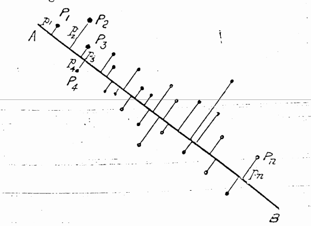
Pearson, 1901: http://stat.smmu.edu.cn/history/pearson1901.pdf

Imagine you have got a set of high dimensional vectors and you want to visualize them in a 3d plot that is helpful to discrimate your data points. With PCA you first find new “axes” for your data which show a lot of variation. They are not related to the metrics on your axes anymore because they form combinations. We call these new “axes” components.

As you can see in the figure from Pearson’s first introduction of the idea in 1901, the points had an x- and y-axis. The first new component is a good line fit through the points which is reduced by the euclidean distance (L²).

The next component can be found by minimizing the L² distance of a line which is perpendicular to the first line and so on.

Only take the first n components of them and you get the principal components n. For the problem with the 3d plot we make n=3.

The last step would be to project all data points from the original coordinate system to the new coordinate system spanned by the three principal components.

An interactive illustration can be found here: http://setosa.io/…

Steps to obtain the principal components

(Taken from https://www.youtube.com/watch?v=fKivxsVlycs)

1. Center the data by substracting the mean
2. Calculate the covariance matrix
3. Find eigenvectors and eigenvalues of the covariance matrix
4. Sort the eigenvectors by their eigenvalues and you obtain the principal components
5. Use matrix multiplication to project the data in the new space

Do it in numpy

(Compare to https://glowingpython.blogspot.de/…)

import numpy as np

1. Center the data (input matrix A) by substracting the mean M = (A - np.mean(A.T, axis=1)).T
2. Calculate the covariance matrix covM = np.cov(M)
3. Find eigenvectors and eigenvalues of the covariance matrix latent, coeff = np.linalg.eig(covM)
4. Sort the eigenvectors by their eigenvalues and you obtain the principal components
   1. Sort the eigenvalues idx = np.argsort(latent)[::-1]
   2. Sort the eigenvectors coeff = coeff[:,idx]
5. Use matrix multiplication to project the data in the new space new_points = np.dot(coeff.T, M)

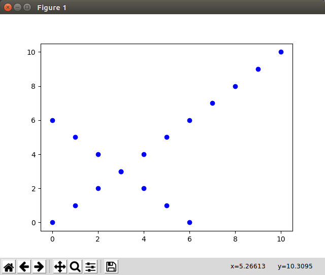
Toy data

Let’s build a toy data set of which we know how pca should align it:

A = array([
    list(range(0, 11)) + list(range(0, 7)),
    list(range(0, 11)) + list(reversed(range(0, 7)))
])

Test PCA: Now we call pca(A.T, target_dimensions=2) and plot the new points

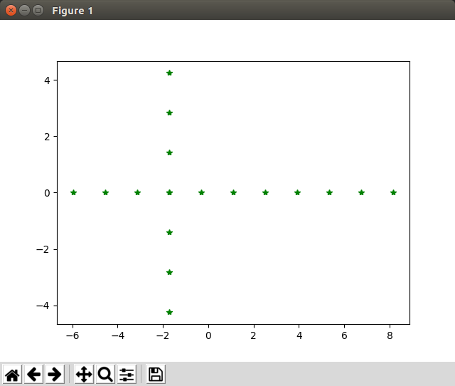
Hooray! Things work as expected!